

Introduction
Every year, Spotify users eagerly await the release of Spotify Wrapped, a personalized year-in-review showcasing their most listened-to songs, artists, and genres. What if I told you there’s a way to get a sneak peek at your Spotify statistics before the official release?
In this guide, I’ll walk you through a Spotify Wrapped hack that allows you to create your own personalized stats using your Spotify streaming data. This way you won’t need to wait for Spotify Wrapped, and you will also be able to create stats that Spotify won’t show you.
Prerequisites
Similar to one of my earlier projects, we will use Jupyter Notebook for this one. It’s a great tool for experimenting and working with data.
If you haven’t installed Jupyter Notebook yet, follow the instructions on their official website. Once installed, you can create a new Jupyter Notebook and get ready for diving into your Spotify stats.
Gathering and Sanitizing Data
To get started, you’ll need to request your Spotify streaming data. You can do this here(make sure you request the “Extended streaming history”). It will take some time for Spotify to send you your data. Requesting only the “Account data” will be faster and will also give you last year’s streaming history. However, it is way less detailed and you will have to adapt the code.
Once you have the data, we can import it. You will get multiple JSON files. Each file consists of an array of objects containing information about a played song or podcast episode:
{
	"ts": "2023-01-30T16:36:40Z",
	"username": "",
	"platform": "linux",
	"ms_played": 239538,
	"conn_country": "DE",
	"ip_addr_decrypted": "",
	"user_agent_decrypted": "",
	"master_metadata_track_name": "Wonderwall - Remastered",
	"master_metadata_album_artist_name": "Oasis",
	"master_metadata_album_album_name": "(What's The Story) Morning Glory? (Deluxe Remastered Edition)",
	"spotify_track_uri": "spotify:track:7ygpwy2qP3NbrxVkHvUhXY",
	"episode_name": null,
	"episode_show_name": null,
	"spotify_episode_uri": null,
	"reason_start": "remote",
	"reason_end": "remote",
	"shuffle": false,
	"skipped": false,
	"offline": false,
	"offline_timestamp": 0,
	"incognito_mode": false
}
This allows you not only to figure out when and on which device you listened to a song but also gives you information such as if and when you skipped it.
We will simply merge all of them into a single Pandas data frame:
path_to_json = 'my_spotify_data/'
frames = []
for file_name in [file for file in os.listdir(path_to_json) if file.endswith('.json')]:
    frames.append(pd.read_json(path_to_json + file_name))

df = pd.concat(frames)
Afterward, we’ll sanitize it by removing podcasts, filtering out short play durations, and converting timestamps to a more readable format:
# drop all rows containing podcasts
df = df[df['spotify_track_uri'].notna()]

# drop all songs which were playing less than 15 seconds
df = df[df['ms_played'] > 15000]

# convert ts from string to datetime
df['ts'] = pd.to_datetime(df['ts'], utc=False)
df['date'] = df['ts'].dt.date

# drop all columns which are not needed
columns_to_keep = [
    'ts',
    'date',
    'ms_played',
    'platform',
    'conn_country',
    'master_metadata_track_name',
    'master_metadata_album_artist_name',
    'master_metadata_album_album_name',
    'spotify_track_uri'
]
df = df[columns_to_keep]

df = df.sort_values(by=['ts'])
songs_df = df.copy()
Analyzing and Visualizing Your Spotify Stats
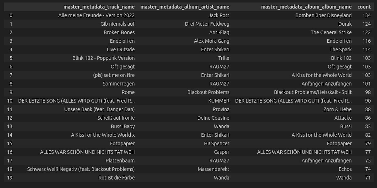
Top Songs of All Time
Let’s kick things off by exploring your all-time favorite songs. We can easily unveil our top tracks based on your streaming history:
df = songs_df.copy()


df = df.groupby(['spotify_track_uri']).size().reset_index().rename(columns={0: 'count'})
df = df.sort_values(by=['count'], ascending=False).reset_index()

df = df.merge(songs_df.drop_duplicates(subset='spotify_track_uri'))
df = df[['master_metadata_track_name', 'master_metadata_album_artist_name', 'master_metadata_album_album_name', 'count']]

df.head(20)
Top Songs in 2023
Curious about this year’s music trends? We can use this function to reveal the top songs of 2023:
def top_songs_in_year(year):
    df = songs_df.copy()

    df['year'] = df['ts'].dt.year

    df = df.loc[(df['year'] == year)]

    print(f"Time listened in {year}: {datetime.timedelta(milliseconds=int(df['ms_played'].sum()))}")

    df = df.groupby(['spotify_track_uri']).size().reset_index().rename(columns={0: 'count'})
    df = df.sort_values(by=['count'], ascending=False).reset_index()

    df = df.merge(songs_df.drop_duplicates(subset='spotify_track_uri'))
    df = df[['master_metadata_track_name',
             'master_metadata_album_artist_name',
             'master_metadata_album_album_name',
             'count']]

    return df.head(20)
My Top Songs 2023
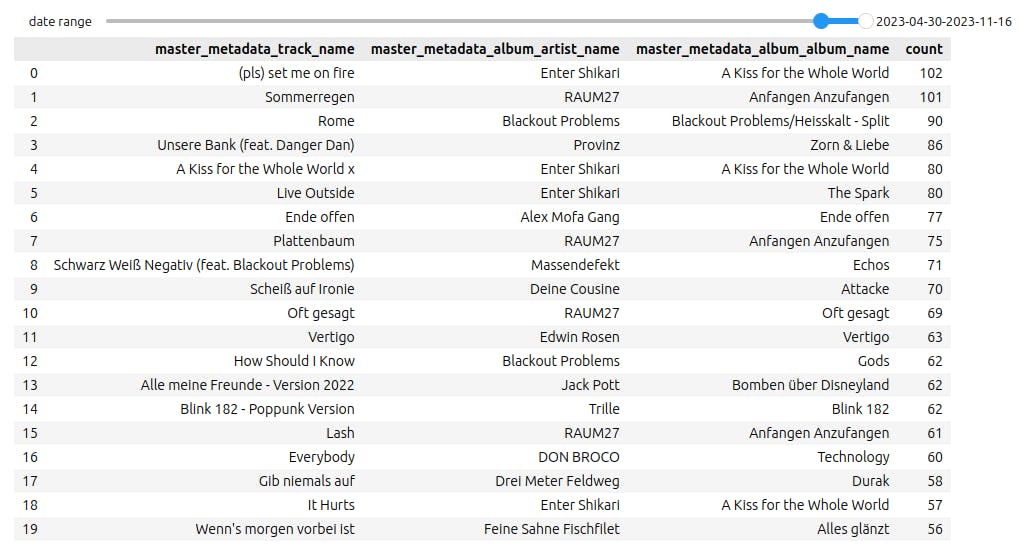
Interactivity With Widgets
That works very well already, but why settle for that? We can use interactive widgets to customize the queries using UI elements. This allows us to find out your top songs in any specific time range effortlessly:
@interact
def top_songs(date_range=date_range_slider):
    df = songs_df.copy()

    time_range_start = pd.Timestamp(date_range[0])
    time_range_end = pd.Timestamp(date_range[1])

    df = df.loc[(df['date'] >= time_range_start.date())
                & (df['date'] <= time_range_end.date())]

    df = df.groupby(['spotify_track_uri']).size().reset_index().rename(columns={0: 'count'})
    df = df.sort_values(by=['count'], ascending=False).reset_index()

    df = df.merge(songs_df.drop_duplicates(subset='spotify_track_uri'))
    df = df[['master_metadata_track_name',
             'master_metadata_album_artist_name',
             'master_metadata_album_album_name',
             'count']]

    return df.head(20)
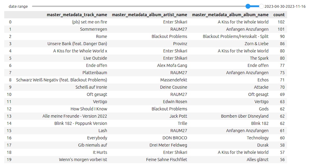
My top songs in the last six months
Temporal and Weekday Distribution
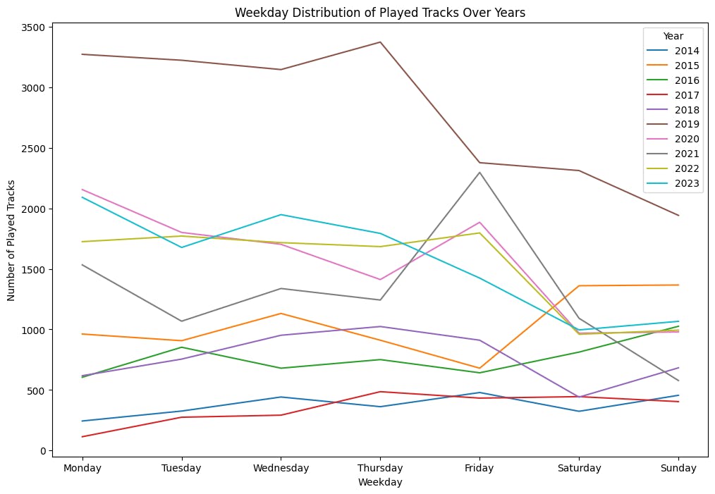
Now that we know our top songs, top artists, and top albums, we can go a little further. For example, exploring which days of the week we’re most active on Spotify:
def plot_weekday_distribution():
    df = songs_df.copy()

    df['year'] = df['ts'].dt.year
    df['weekday'] = df['ts'].dt.weekday

    df = df.groupby(['year', 'weekday']).size().reset_index(name='count')

    fig, ax = plt.subplots(figsize=(12, 8))

    for year, data in df.groupby('year'):
        ax.plot(data['weekday'], data['count'], label=str(year))

    weekdays_order = ['Monday', 'Tuesday', 'Wednesday', 'Thursday', 'Friday', 'Saturday', 'Sunday']
    plt.xticks(range(7), weekdays_order)

    plt.title('Weekday Distribution of Played Tracks Over Years')
    plt.xlabel('Weekday')
    plt.ylabel('Number of Played Tracks')
    plt.legend(title='Year')

    plt.show()
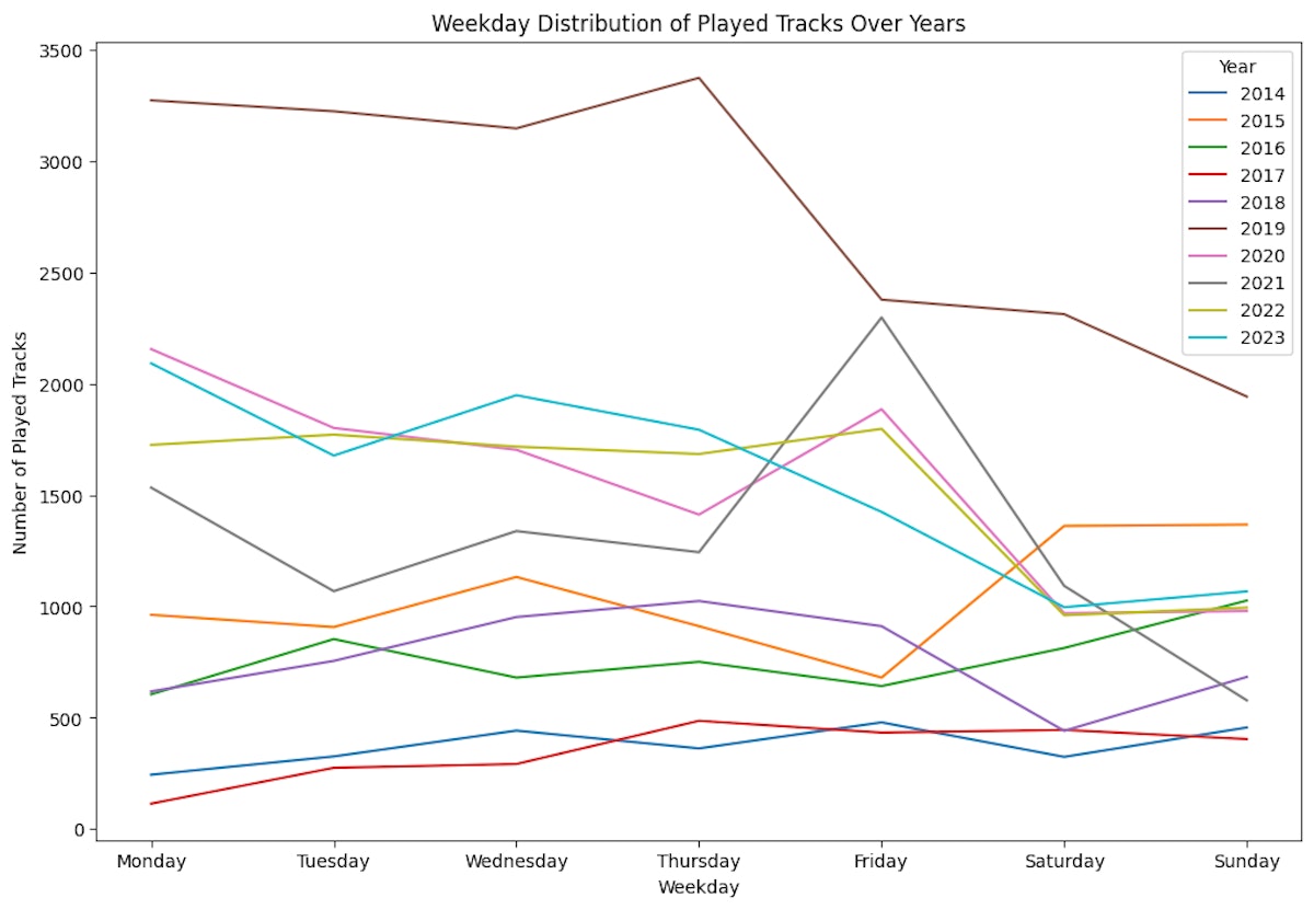
My weekday distribution
How to Do It Yourself
Ready to dive into your own Spotify stats? Check out my GitHub repository to find all the code, including even more functions to explore your listening stats.
Conclusion
Creating your Spotify stats before the official release not only adds an element of fun but also provides insights into your unique listening habits. As we eagerly anticipate Spotify Wrapped, why not get a head start on your music analysis adventure?
Get ready to groove into your personalized Spotify Wrapped experience!
This article was originally published by Lukas Krimphove on Hackernoon.


